
- Mathematics in Marketing: Statistics is essential for deciphering patterns and predicting sales based on campaign data.
- Simple Linear Regression: Uses an independent variable (such as marketing spending) to predict a dependent variable (sales), represented by a straight line.
- Multiple Linear Regression: It considers multiple factors, such as price and economy, to create more accurate and robust forecasts, capturing the complexity of the market.
Mathematics as a Marketing Language
Since ancient times, mathematics has been seen as the language of the universe, capable of describing everything from the movement of planets to the growth of plants. In the marketing context, mathematics allows us to decipher hidden patterns in the endless amounts of data generated by advertising campaigns, mainly through statistics. Next, we explain one of the main numerical tools that structure a Marketing Mix Modeling analysis, Regression.
- Also read: Introduction to Marketing Mix Modeling (MMM)
Linear Regression: The Simplicity of the Line
The MMM is both an analysis and a prediction. At the end of the day, what we want to do is estimate values that could not initially be predicted. In statistics, the simplest and most didactic tool to do this work is linear regression. Regression is an equation for estimating the expected value of a variable And, given the values of some other variables x.
Let's, as an example, create a very basic model, where we use marketing spending data to predict future sales with a simple linear regression.
Example: A relationship between investment and sales
Using fictitious 12-month data, we can try to predict sales for the next 3 months based on marketing spending.
And now let's assume the following marketing spending for the next 3 months:
Finally, we used linear regression to predict sales for months 13, 14, and 15
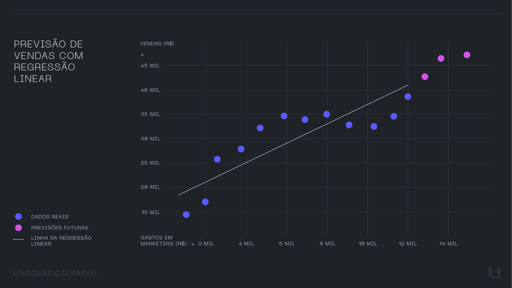
Blue Dots: They represent actual marketing and sales spending data for the initial 12 months.
Linha: Represents the linear regression line adjusted to the data.
Purple Dots: Represent sales forecasts for months 13, 14, and 15 based on expected marketing expenses.
Simple linear regression follows the formula:
Y = β0 + β1x
Where:
AND It is the amount of expected sales
beta0 It's the constant
Beta-1 It is the slope coefficient
X It is the independent variable (marketing spending)
You can try doing a simple regression with your marketing and sales data, using the command FORECAST.LINEAR not Excel.
Incorporating Multiple Factors
While simple linear regression is useful for predicting a dependent variable (such as sales) based on a single independent variable (such as marketing spending), in reality, in MMM we calculate the influence of multiple factors. To capture this complexity, we used multiple linear regression.
In multiple linear regression, we consider several independent variables (for example, marketing spending, product price, economic conditions) to predict the dependent variable (sales). The multiple linear regression formula is an extension of the simple linear regression formula and can be written like this:
Y = beta-0 + B-1x1 + B-2x2 + B-3x3 +
Where:
AND Are the expected sales
X1 Are marketing expenses
X2 It's the price of the product
X3 It is the economic growth rate
bet0, bet1, bet2, bet3They are the model coefficients and are the error
By using multiple linear regression, we can predict sales taking into account not only marketing spending, but also other factors that may influence the result. This makes forecasts more robust and accurate, better reflecting the complex reality of the market.
Practical Example of Multiple Linear Regression:
Suppose that, in addition to marketing spending, we also have data on the price of the product and the economic growth rate over the past 12 months. We can use these three factors to create a multiple linear regression model that predicts sales for the next 3 months. The adjusted formula would be:
Y = β0 + β1 (Marketing Expenses) + β2 (Product Price) + β3 (Economic Growth) +
Let's then create another set of fictitious data for the variables mentioned, considering three independent variables (marketing spending, product price, and economic growth rate) to predict a dependent variable (sales).
Marketing Expenses (X1): In millions of reais
Product Price (X2): In reais
Economic Growth Rate (X3): In percentage
Sales (Y): In millions of units
How are the Coefficients of the formula Calculated?
The coefficients are calculated using the least squares method. This method adjusts the line that minimizes the sum of the squares of the differences between the real values and the values predicted by the model. The calculation of the coefficients involves the following steps:
Organize the data in an array.
Multiply the data matrix by its transpose.
Calculate the inverse of the resulting matrix.
Multiply the result by the vector of observed values (sales).
The Excel linear regression function does this calculation automatically. See PROJ.LIN
Calculated Coefficients
Based on the calculations, the coefficients of the multiple linear regression equation are:
beta0 = 28.04
Beta-1 = 4.58 (for Marketing Spending)
beta2= −0.12 (for Product Price)
beta-3 = 1.64 (for Economic Growth Rate)
Thus, the regression equation for predicting sales (Y) is:
Y = 28.04 + 4.58×X1 −0.12×X2 + 1.64×X3
Forecast for the Next 3 Months
Now, let's forecast sales for the next 3 months, assuming that we have the following future conditions:
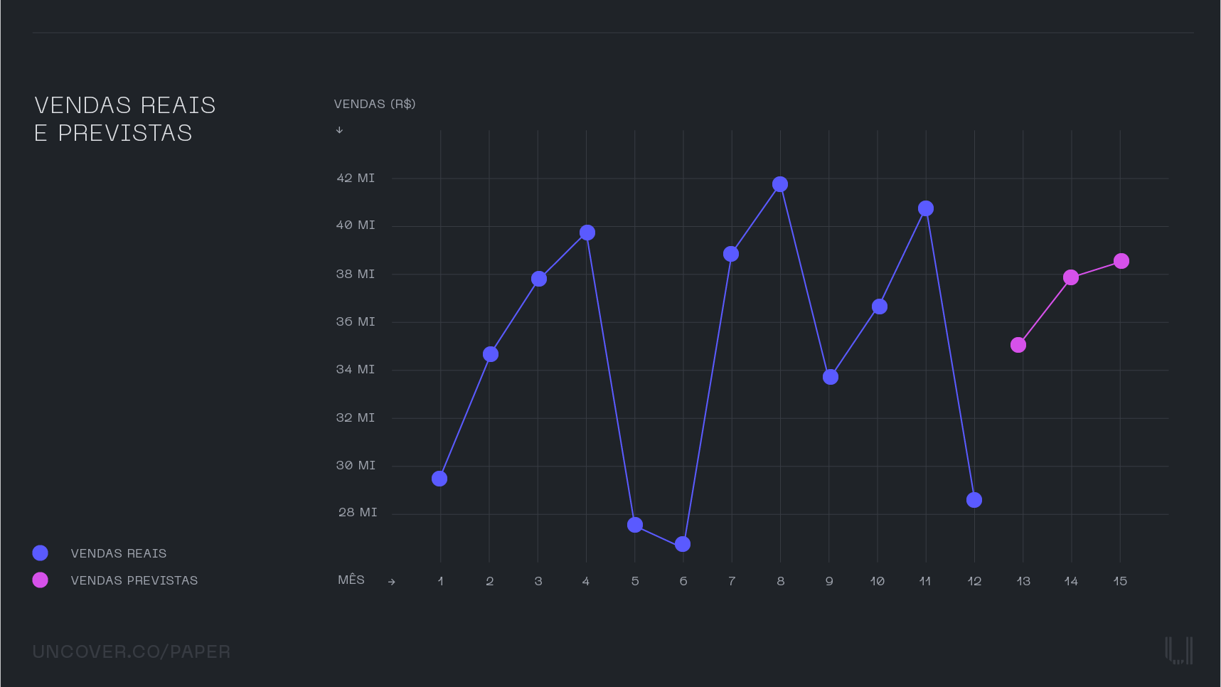
Forecast Results
The sales forecasts for the next 3 months are:
Month 13: 35.41 million units
Month 14: 37.93 million units
Month 15: 38.44 million units
Incorporating the Error
The error term α represents the difference between the actual observed sales value Y and the value predicted by the regression model. The error captures the variations in the data that are not explained by the independent variables included in the model.
= Y (real) - Y
The error may be caused by:
Factors not included in the model: As the model only takes into account marketing spending, product price, and economic growth rate, any other factor that influences sales (such as seasonality, changes in consumer behavior, etc.) will be caught in the error.
Random noise: Small variations that occur naturally in the data and do not follow a specific pattern.
Error Forecasting and Calculation
Suppose that for month 13, the variable values are:
Marketing Spending (X1) = 3.2
Product Price (X2) = 101
Economic Growth Rate (X3) = 2.9
Using the equation, the prediction would be:
Y13 = 25+3.5 (3.2) − 0.2 (101) +1.8 (2.9) = 34.46 units
If the actual sales in month 13 were 36 units, the error would be:
13 = Yreal − Y = 36 − 34.46 = 1.54 units
Conclusion
The error is a fundamental part of regression analysis, as it represents the variations that the model failed to capture. It helps us understand the accuracy of the model and identify areas where it can be improved. By analyzing errors in a systematic way, the company can adjust its strategies and improve its future forecasts.